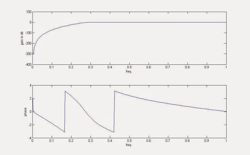
This mini project introduces a new class of IIR digital filters.That unifies the classical digital Butterworth High Pass filter. New closed form expressions are provided, and a straight forward design technique is described. The new IIR digital filters have non linear phase & more zeros than poles (away from the origin) and their (monotonic) square magnitude frequency responses are maximally flat w= 0 and at w =pi. This technique also permits continuous variation of the cut-off frequency.
We can also use Digital signal processor DSP Microcontroller like DSPPic from Microchip technology,TMS320C5000 series DSP controller from TI Texas Instruments etc.
The Butterworth High Pass Filter attenuates all frequencies below cut-off frequency and passes all frequencies above cut-off frequency.
 |
| Butterworth_High_Pass_Filter_DSP_MATLAB www.beprojectidea.blogspot.com |
Aim:
Design Butterworth Highpass filter using MATLAB.Theory:
This introduction makes
the link with analog filters and associated frequency transformation.
The digital filters are simply computed from the analog transfer
functions using the bi linear transform.
A key element in processing digital signals is the filter. Filters perform direct Manipulations on the spectra of signals. To completely describe digital filters, three basic elements (or building blocks) are needed: an adder, a multiplier, and a delay element. The adder has two inputs and one output, and it simply adds the two inputs together. The multiplier is a gain element, and it multiplies the input signal by a constant. The delay element delays the incoming signal by one sample. Digital filters can be implemented using either a block diagram or a signal flow graph. Figure 1 shows the three basic elements in block diagram form, and Figure 2 shows them in signal flow graph form.
A key element in processing digital signals is the filter. Filters perform direct Manipulations on the spectra of signals. To completely describe digital filters, three basic elements (or building blocks) are needed: an adder, a multiplier, and a delay element. The adder has two inputs and one output, and it simply adds the two inputs together. The multiplier is a gain element, and it multiplies the input signal by a constant. The delay element delays the incoming signal by one sample. Digital filters can be implemented using either a block diagram or a signal flow graph. Figure 1 shows the three basic elements in block diagram form, and Figure 2 shows them in signal flow graph form.
 | |||||||||
| Block Diagram of Butterworth High pass filter using MATLAB Element |
 |
| Signal Flow Graph of Filter Elements (Digital Signal Processing (DSP) Butterworth HighPass Filter ) |
With the basic building blocks at hand, the two different filter structures can easily be implemented. These two structures are Infinite Impulse Response (IIR) and Finite Impulse Response (FIR), depending on the form of the system’s response to a unit pulse input. IIR filters are commonly implemented using a feedback (recursive) structure; while FIR filters usually require no feedback (non-recursive).
In the design of IIR filters, a commonly used approach is called the bilinear transformation. This design begins with the transfer function of an analog filter, and then performs a mapping from the s-domain to the z-domain. Using differential equations, it can be shown (Proakis 677) that the mapping from the s-plane to the z-plane is
 |
| mapping from the s-plane to the z-plane |
This mapping results in a general form for an IIR filter with an arbitrary number of poles and zeros. The system response and the difference equation for this filter are as follows:
 |
| system response and the difference equation for an IIR filter |
This system response can be easily realized using a signal flow graph.


